Instruction

Addition method.
You need to write two strictly under each other:

549+45y+4y=-7, 45y+4y=549-7, 49y=542, y=542:49, y≈11.
In an arbitrarily chosen (from the system) equation, insert the number 11 instead of the already found "game" and calculate the second unknown:

X=61+5*11, x=61+55, x=116.
The answer of this system of equations: x=116, y=11.

Graphic way.
It consists in the practical finding of the coordinates of the point at which the lines are mathematically written in the system of equations. You should draw graphs of both lines separately in the same coordinate system. General view: - y \u003d kx + b. To construct a straight line, it is enough to find the coordinates of two points, and x is chosen arbitrarily.
Let the system be given: 2x - y \u003d 4

Y \u003d -3x + 1.
A straight line is built according to the first one, for convenience it needs to be written down: y \u003d 2x-4. Come up with (easier) values ​​for x, substituting it into the equation, solving it, find y. Two points are obtained, along which a straight line is built. (see pic.)
x 0 1

y -4 -2
A straight line is constructed according to the second equation: y \u003d -3x + 1.
Also build a line. (see pic.)

1-5
Find the coordinates of the intersection point of two constructed lines on the graph (if the lines do not intersect, then the system of equations does not have - so).

Related videos

Useful advice

If the same system of equations is solved in three different ways, the answer will be the same (if the solution is correct).

Sources:

• Algebra Grade 8
• solve an equation with two unknowns online
• Examples of solving systems of linear equations with two

System equations is a collection of mathematical records, each of which contains a certain number of variables. There are several ways to solve them.

You will need

• -Ruler and pencil;
• -calculator.

Instruction

Consider the sequence of solving the system, which consists of linear equations having the form: a1x + b1y = c1 and a2x + b2y = c2. Where x and y are unknown variables and b,c are free members. When applying this method, each system is the coordinates of the points corresponding to each equation. First, in each case, express one variable in terms of the other. Then set the x variable to any number of values. Two is enough. Plug into the equation and find y. Build a coordinate system, mark the obtained points on it and draw a straight line through them. Similar calculations must be carried out for other parts of the system.

The system has a unique solution if the constructed lines intersect and have one common point. It is inconsistent if they are parallel to each other. And it has infinitely many solutions when the lines merge with each other.

This method is considered to be very clear. The main disadvantage is that the calculated unknowns have approximate values. A more accurate result is given by the so-called algebraic methods.

Any solution to a system of equations is worth checking. To do this, substitute the obtained values ​​instead of the variables. You can also find its solution in several ways. If the solution of the system is correct, then everyone should turn out the same.

Often there are equations in which one of the terms is unknown. To solve an equation, you need to remember and do a certain set of actions with these numbers.

You will need

• - paper;
• - Pen or pencil.

Instruction

Imagine that you have 8 rabbits in front of you, and you only have 5 carrots. Think you need to buy more carrots so that each rabbit gets a carrot.

Let's represent this problem in the form of an equation: 5 + x = 8. Let's substitute the number 3 for x. Indeed, 5 + 3 = 8.

When you substituted a number for x, you were doing the same operation as subtracting 5 from 8. Thus, to find unknown term, subtract the known term from the sum.

Let's say you have 20 rabbits and only 5 carrots. Let's compose . An equation is an equality that holds only for certain values ​​of the letters included in it. The letters whose values ​​you want to find are called. Write an equation with one unknown, call it x. When solving our problem about rabbits, the following equation is obtained: 5 + x = 20.

Let's find the difference between 20 and 5. When subtracting, the number from which it is subtracted is reduced. The number that is subtracted is called , and the final result is called the difference. So, x = 20 - 5; x = 15. You need to buy 15 carrots for rabbits.

Make a check: 5 + 15 = 20. The equation is correct. Of course, when it comes to such simple , the check is not necessary. However, when it comes to equations with three-digit, four-digit, and so on, it is imperative to perform a check in order to be absolutely sure of the result of your work.

Related videos

Useful advice

To find the unknown minuend, you need to add the subtrahend to the difference.

To find the unknown subtrahend, it is necessary to subtract the difference from the minuend.

Tip 4: How to solve a system of three equations with three unknowns

A system of three equations with three unknowns may not have solutions, despite a sufficient number of equations. You can try to solve it using the substitution method or using the Cramer method. Cramer's method, in addition to solving the system, allows one to evaluate whether the system is solvable before finding the values ​​of the unknowns.

Instruction

The substitution method consists in sequentially one unknown through two others and substituting the result obtained into the equations of the system. Let a system of three equations be given in general form:

a1x + b1y + c1z = d1

a2x + b2y + c2z = d2

a3x + b3y + c3z = d3

Express x from the first equation: x = (d1 - b1y - c1z)/a1 - and substitute into the second and third equations, then express y from the second equation and substitute into the third. You will get a linear expression for z through the coefficients of the equations of the system. Now go "back": plug z into the second equation and find y, then plug z and y into the first equation and find x. The process is generally shown in the figure until z is found. Further, the record in general form will be too cumbersome, in practice, substituting , you can quite easily find all three unknowns.

Cramer's method consists in compiling the matrix of the system and calculating the determinant of this matrix, as well as three more auxiliary matrices. The matrix of the system is composed of the coefficients at the unknown terms of the equations. The column containing the numbers on the right side of the equations, the column of the right side. It is not used in the system, but is used when solving the system.

Related videos

note

All equations in the system must supply additional information independent of other equations. Otherwise, the system will be underdetermined and it will not be possible to find an unambiguous solution.

Useful advice

After solving the system of equations, substitute the found values ​​into the original system and check that they satisfy all the equations.

By itself the equation with three unknown has many solutions, so most often it is supplemented by two more equations or conditions. Depending on what the initial data are, the course of the decision will largely depend.

You will need

• - a system of three equations with three unknowns.

Instruction

If two of the three systems have only two of the three unknowns, try expressing some variables in terms of the others and plugging them into the equation with three unknown. Your goal with this is to turn it into a normal the equation with the unknown. If this is , the further solution is quite simple - substitute the found value into other equations and find all the other unknowns.

Some systems of equations can be subtracted from one equation by another. See if it is possible to multiply one of by or a variable so that two unknowns are reduced at once. If there is such an opportunity, use it, most likely, the subsequent decision will not be difficult. Do not forget that when multiplying by a number, you must multiply both the left side and the right side. Similarly, when subtracting equations, remember that the right hand side must also be subtracted.

If the previous methods did not help, use the general method for solving any equations with three unknown. To do this, rewrite the equations in the form a11x1 + a12x2 + a13x3 \u003d b1, a21x1 + a22x2 + a23x3 \u003d b2, a31x1 + a32x2 + a33x3 \u003d b3. Now make a matrix of coefficients at x (A), a matrix of unknowns (X) and a matrix of free ones (B). Pay attention, multiplying the matrix of coefficients by the matrix of unknowns, you will get a matrix, a matrix of free members, that is, A * X \u003d B.

Find the matrix A to the power (-1) after finding , note that it should not be equal to zero. After that, multiply the resulting matrix by matrix B, as a result you will get the desired matrix X, indicating all the values.

You can also find a solution to a system of three equations using the Cramer method. To do this, find the third-order determinant ∆ corresponding to the matrix of the system. Then successively find three more determinants ∆1, ∆2 and ∆3, substituting the values ​​of the free terms instead of the values ​​of the corresponding columns. Now find x: x1=∆1/∆, x2=∆2/∆, x3=∆3/∆.

Sources:

• solutions of equations with three unknowns

Starting to solve a system of equations, figure out what these equations are. The methods of solving linear equations are well studied. Nonlinear equations are most often not solved. There are only one special cases, each of which is practically individual. Therefore, the study of methods of solution should begin with linear equations. Such equations can be solved even purely algorithmically.

the denominators of the found unknowns are exactly the same. Yes, and the numerators are visible some patterns of their construction. If the dimension of the system of equations were greater than two, then the elimination method would lead to very cumbersome calculations. To avoid them, purely algorithmic solutions have been developed. The simplest of them is Cramer's algorithm (Cramer's formulas). For should learn the general system of equations of n equations.

The system of n linear algebraic equations with n unknowns has the form (see Fig. 1a). In it, aij are the coefficients of the system,
хj – unknowns, bi – free members (i=1, 2, ... , n; j=1, 2, ... , n). Such a system can be compactly written in the matrix form AX=B. Here A is the coefficient matrix of the system, X is the column matrix of unknowns, B is the column matrix of free terms (see Fig. 1b). According to Cramer's method, each unknown xi =∆i/∆ (i=1,2…,n). The determinant ∆ of the matrix of coefficients is called the main determinant, and ∆i is called auxiliary. For each unknown, an auxiliary determinant is found by replacing the i-th column of the main determinant with a column of free members. Cramer's method for the case of systems of the second and third order is presented in detail in Fig. 2.

A system is a union of two or more equalities, each of which has two or more unknowns. There are two main ways to solve systems of linear equations that are used in the school curriculum. One of them is called the method, the other is the addition method.

Standard form of a system of two equations

In standard form, the first equation is a1*x+b1*y=c1, the second equation is a2*x+b2*y=c2, and so on. For example, in the case of two parts of the system in both given a1, a2, b1, b2, c1, c2 are some numerical coefficients presented in specific equations. In turn, x and y are unknowns whose values ​​need to be determined. The desired values ​​turn both equations simultaneously into true equalities.

Solution of the system by the addition method

In order to solve the system, that is, to find those values ​​of x and y that will turn them into true equalities, you need to take a few simple steps. The first of these is to transform any of the equations in such a way that the numerical coefficients for the variable x or y in both equations coincide in absolute value, but differ in sign.

For example, let a system consisting of two equations be given. The first of them has the form 2x+4y=8, the second has the form 6x+2y=6. One of the options for completing the task is to multiply the second equation by a factor of -2, which will lead it to the form -12x-4y=-12. The correct choice of the coefficient is one of the key tasks in the process of solving the system by the addition method, since it determines the entire further course of the procedure for finding unknowns.

Now it is necessary to add the two equations of the system. Obviously, the mutual destruction of variables with equal in value but opposite in sign coefficients will lead it to the form -10x=-4. After that, it is necessary to solve this simple equation, from which it unambiguously follows that x=0.4.

The last step in the solution process is the substitution of the found value of one of the variables into any of the initial equalities available in the system. For example, substituting x=0.4 into the first equation, you can get the expression 2*0.4+4y=8, from which y=1.8. Thus, x=0.4 and y=1.8 are the roots of the system shown in the example.

In order to make sure that the roots were found correctly, it is useful to check by substituting the found values ​​into the second equation of the system. For example, in this case, an equality of the form 0.4 * 6 + 1.8 * 2 = 6 is obtained, which is correct.

Related videos

Let us first recall the definition of a solution to a system of equations in two variables.

Definition 1

A pair of numbers is called a solution to a system of equations with two variables if, when they are substituted into the equation, the correct equality is obtained.

In what follows, we will consider systems of two equations with two variables.

Exist four basic ways to solve systems of equations: substitution method, addition method, graphical method, new variable management method. Let's look at these methods with specific examples. To describe the principle of using the first three methods, we will consider a system of two linear equations with two unknowns:

Substitution method

The substitution method is as follows: any of these equations is taken and $y$ is expressed in terms of $x$, then $y$ is substituted into the equation of the system, from where the variable $x.$ is found. After that, we can easily calculate the variable $y.$

Example 1

Let us express from the second equation $y$ in terms of $x$:

Substitute in the first equation, find $x$:

\ \ \

Find $y$:

Answer: $(-2,\ 3)$

Addition method.

Consider this method with an example:

Example 2

\[\left\( \begin(array)(c) (2x+3y=5) \\ (3x-y=-9) \end(array) \right.\]

Multiply the second equation by 3, we get:

\[\left\( \begin(array)(c) (2x+3y=5) \\ (9x-3y=-27) \end(array) \right.\]

Now let's add both equations together:

\ \ \

Find $y$ from the second equation:

\[-6-y=-9\] \

Answer: $(-2,\ 3)$

Remark 1

Note that in this method it is necessary to multiply one or both equations by such numbers that when adding one of the variables "disappears".

Graphical way

The graphical method is as follows: both equations of the system are displayed on the coordinate plane and the point of their intersection is found.

Example 3

\[\left\( \begin(array)(c) (2x+3y=5) \\ (3x-y=-9) \end(array) \right.\]

Let us express $y$ from both equations in terms of $x$:

\[\left\( \begin(array)(c) (y=\frac(5-2x)(3)) \\ (y=3x+9) \end(array) \right.\]

Let's draw both graphs on the same plane:

Picture 1.

Answer: $(-2,\ 3)$

How to introduce new variables

We will consider this method in the following example:

Example 4

\[\left\( \begin(array)(c) (2^(x+1)-3^y=-1) \\ (3^y-2^x=2) \end(array) \right .\]

Solution.

This system is equivalent to the system

\[\left\( \begin(array)(c) ((2\cdot 2)^x-3^y=-1) \\ (3^y-2^x=2) \end(array) \ right.\]

Let $2^x=u\ (u>0)$ and $3^y=v\ (v>0)$, we get:

\[\left\( \begin(array)(c) (2u-v=-1) \\ (v-u=2) \end(array) \right.\]

We solve the resulting system by the addition method. Let's add the equations:

\ \

Then from the second equation, we get that

Returning to the replacement, we obtain a new system of exponential equations:

\[\left\( \begin(array)(c) (2^x=1) \\ (3^y=3) \end(array) \right.\]

We get:

\[\left\( \begin(array)(c) (x=0) \\ (y=1) \end(array) \right.\]

Solving systems of linear algebraic equations (SLAE) is undoubtedly the most important topic of the linear algebra course. A huge number of problems from all branches of mathematics are reduced to solving systems of linear equations. These factors explain the reason for creating this article. The material of the article is selected and structured so that with its help you can

• choose the optimal method for solving your system of linear algebraic equations,
• study the theory of the chosen method,
• solve your system of linear equations, having considered in detail the solutions of typical examples and problems.

Brief description of the material of the article.

First, we give all the necessary definitions, concepts, and introduce some notation.

Next, we consider methods for solving systems of linear algebraic equations in which the number of equations is equal to the number of unknown variables and which have a unique solution. First, let's focus on the Cramer method, secondly, we will show the matrix method for solving such systems of equations, and thirdly, we will analyze the Gauss method (the method of successive elimination of unknown variables). To consolidate the theory, we will definitely solve several SLAEs in various ways.

After that, we turn to solving systems of linear algebraic equations of a general form, in which the number of equations does not coincide with the number of unknown variables or the main matrix of the system is degenerate. We formulate the Kronecker-Capelli theorem, which allows us to establish the compatibility of SLAEs. Let us analyze the solution of systems (in the case of their compatibility) using the concept of the basis minor of a matrix. We will also consider the Gauss method and describe in detail the solutions of the examples.

Be sure to dwell on the structure of the general solution of homogeneous and inhomogeneous systems of linear algebraic equations. Let us give the concept of a fundamental system of solutions and show how the general solution of the SLAE is written using the vectors of the fundamental system of solutions. For a better understanding, let's look at a few examples.

In conclusion, we consider systems of equations that are reduced to linear ones, as well as various problems, in the solution of which SLAEs arise.

Page navigation.

Definitions, concepts, designations.

We will consider systems of p linear algebraic equations with n unknown variables (p may be equal to n ) of the form

Unknown variables, - coefficients (some real or complex numbers), - free members (also real or complex numbers).

This form of SLAE is called coordinate.

AT matrix form this system of equations has the form ,
where - the main matrix of the system, - the matrix-column of unknown variables, - the matrix-column of free members.

If we add to the matrix A as the (n + 1)-th column the matrix-column of free terms, then we get the so-called expanded matrix systems of linear equations. Usually, the augmented matrix is ​​denoted by the letter T, and the column of free members is separated by a vertical line from the rest of the columns, that is,

By solving a system of linear algebraic equations called a set of values ​​of unknown variables , which turns all the equations of the system into identities. The matrix equation for the given values ​​of the unknown variables also turns into an identity.

If a system of equations has at least one solution, then it is called joint.

If the system of equations has no solutions, then it is called incompatible.

If a SLAE has a unique solution, then it is called certain; if there is more than one solution, then - uncertain.

If the free terms of all equations of the system are equal to zero , then the system is called homogeneous, otherwise - heterogeneous.

Solution of elementary systems of linear algebraic equations.

If the number of system equations is equal to the number of unknown variables and the determinant of its main matrix is ​​not equal to zero, then we will call such SLAEs elementary. Such systems of equations have a unique solution, and in the case of a homogeneous system, all unknown variables are equal to zero.

We started studying such SLAE in high school. When solving them, we took one equation, expressed one unknown variable in terms of others and substituted it into the remaining equations, then took the next equation, expressed the next unknown variable and substituted it into other equations, and so on. Or they used the addition method, that is, they added two or more equations to eliminate some unknown variables. We will not dwell on these methods in detail, since they are essentially modifications of the Gauss method.

The main methods for solving elementary systems of linear equations are the Cramer method, the matrix method and the Gauss method. Let's sort them out.

Solving systems of linear equations by Cramer's method.

Let us need to solve a system of linear algebraic equations

in which the number of equations is equal to the number of unknown variables and the determinant of the main matrix of the system is different from zero, that is, .

Let be the determinant of the main matrix of the system, and are determinants of matrices that are obtained from A by replacing 1st, 2nd, …, nth column respectively to the column of free members:

With such notation, the unknown variables are calculated by the formulas of Cramer's method as . This is how the solution of a system of linear algebraic equations is found by the Cramer method.

Example.

Cramer method .

Solution.

The main matrix of the system has the form . Calculate its determinant (if necessary, see the article):

Since the determinant of the main matrix of the system is nonzero, the system has a unique solution that can be found by Cramer's method.

Compose and calculate the necessary determinants (the determinant is obtained by replacing the first column in matrix A with a column of free members, the determinant - by replacing the second column with a column of free members, - by replacing the third column of matrix A with a column of free members):

Finding unknown variables using formulas :

Answer:

The main disadvantage of Cramer's method (if it can be called a disadvantage) is the complexity of calculating the determinants when the number of system equations is more than three.

Solving systems of linear algebraic equations by the matrix method (using the inverse matrix).

Let the system of linear algebraic equations be given in matrix form , where the matrix A has dimension n by n and its determinant is nonzero.

Since , then the matrix A is invertible, that is, there is an inverse matrix . If we multiply both parts of the equality by on the left, then we get a formula for finding the column matrix of unknown variables. So we got the solution of the system of linear algebraic equations by the matrix method.

Example.

Solve System of Linear Equations matrix method.

Solution.

Let's rewrite the system of equations in matrix form:

Because

then the SLAE can be solved by the matrix method. Using the inverse matrix, the solution to this system can be found as .

Let's build an inverse matrix using a matrix of algebraic complements of the elements of matrix A (if necessary, see the article):

It remains to calculate - the matrix of unknown variables by multiplying the inverse matrix on the matrix-column of free members (if necessary, see the article):

Answer:

or in another notation x 1 = 4, x 2 = 0, x 3 = -1.

The main problem in finding solutions to systems of linear algebraic equations by the matrix method is the complexity of finding the inverse matrix, especially for square matrices of order higher than the third.

Solving systems of linear equations by the Gauss method.

Suppose we need to find a solution to a system of n linear equations with n unknown variables
the determinant of the main matrix of which is different from zero.

The essence of the Gauss method consists in the successive exclusion of unknown variables: first, x 1 is excluded from all equations of the system, starting from the second, then x 2 is excluded from all equations, starting from the third, and so on, until only the unknown variable x n remains in the last equation. Such a process of transforming the equations of the system for the successive elimination of unknown variables is called direct Gauss method. After the forward run of the Gauss method is completed, x n is found from the last equation, x n-1 is calculated from the penultimate equation using this value, and so on, x 1 is found from the first equation. The process of calculating unknown variables when moving from the last equation of the system to the first is called reverse Gauss method.

Let us briefly describe the algorithm for eliminating unknown variables.

We will assume that , since we can always achieve this by rearranging the equations of the system. We exclude the unknown variable x 1 from all equations of the system, starting from the second one. To do this, add the first equation multiplied by to the second equation of the system, add the first multiplied by to the third equation, and so on, add the first multiplied by to the nth equation. The system of equations after such transformations will take the form

where , a .

We would come to the same result if we expressed x 1 in terms of other unknown variables in the first equation of the system and substituted the resulting expression into all other equations. Thus, the variable x 1 is excluded from all equations, starting from the second.

Next, we act similarly, but only with a part of the resulting system, which is marked in the figure

To do this, add the second equation multiplied by to the third equation of the system, add the second multiplied by to the fourth equation, and so on, add the second multiplied by to the nth equation. The system of equations after such transformations will take the form

where , a . Thus, the variable x 2 is excluded from all equations, starting from the third.

Next, we proceed to the elimination of the unknown x 3, while acting similarly with the part of the system marked in the figure

So we continue the direct course of the Gauss method until the system takes the form

From this moment, we begin the reverse course of the Gauss method: we calculate x n from the last equation as , using the obtained value of x n we find x n-1 from the penultimate equation, and so on, we find x 1 from the first equation.

Example.

Solve System of Linear Equations Gaussian method.

Solution.

Let's exclude the unknown variable x 1 from the second and third equations of the system. To do this, to both parts of the second and third equations, we add the corresponding parts of the first equation, multiplied by and by, respectively:

Now we exclude x 2 from the third equation by adding to its left and right parts the left and right parts of the second equation, multiplied by:

On this, the forward course of the Gauss method is completed, we begin the reverse course.

From the last equation of the resulting system of equations, we find x 3:

From the second equation we get .

From the first equation we find the remaining unknown variable and this completes the reverse course of the Gauss method.

Answer:

X 1 \u003d 4, x 2 \u003d 0, x 3 \u003d -1.

Solving systems of linear algebraic equations of general form.

In the general case, the number of equations of the system p does not coincide with the number of unknown variables n:

Such SLAEs may have no solutions, have a single solution, or have infinitely many solutions. This statement also applies to systems of equations whose main matrix is ​​square and degenerate.

Kronecker-Capelli theorem.

Before finding a solution to a system of linear equations, it is necessary to establish its compatibility. The answer to the question when SLAE is compatible, and when it is incompatible, gives Kronecker–Capelli theorem:
for a system of p equations with n unknowns (p can be equal to n ) to be consistent it is necessary and sufficient that the rank of the main matrix of the system is equal to the rank of the extended matrix, that is, Rank(A)=Rank(T) .

Let us consider the application of the Kronecker-Capelli theorem to determine the compatibility of a system of linear equations as an example.

Example.

Find out if the system of linear equations has solutions.

Solution.

. Let us use the method of bordering minors. Minor of the second order different from zero. Let's go over the third-order minors surrounding it:

Since all bordering third-order minors are equal to zero, the rank of the main matrix is ​​two.

In turn, the rank of the augmented matrix is equal to three, since the minor of the third order

different from zero.

In this way, Rang(A) , therefore, according to the Kronecker-Capelli theorem, we can conclude that the original system of linear equations is inconsistent.

Answer:

There is no solution system.

So, we have learned to establish the inconsistency of the system using the Kronecker-Capelli theorem.

But how to find the solution of the SLAE if its compatibility is established?

To do this, we need the concept of the basis minor of a matrix and the theorem on the rank of a matrix.

The highest order minor of the matrix A, other than zero, is called basic.

It follows from the definition of the basis minor that its order is equal to the rank of the matrix. For a non-zero matrix A, there can be several basic minors; there is always one basic minor.

For example, consider the matrix .

All third-order minors of this matrix are equal to zero, since the elements of the third row of this matrix are the sum of the corresponding elements of the first and second rows.

The following minors of the second order are basic, since they are nonzero

Minors are not basic, since they are equal to zero.

Matrix rank theorem.

If the rank of a matrix of order p by n is r, then all elements of the rows (and columns) of the matrix that do not form the chosen basis minor are linearly expressed in terms of the corresponding elements of the rows (and columns) that form the basis minor.

What does the matrix rank theorem give us?

If, by the Kronecker-Capelli theorem, we have established the compatibility of the system, then we choose any basic minor of the main matrix of the system (its order is equal to r), and exclude from the system all equations that do not form the chosen basic minor. The SLAE obtained in this way will be equivalent to the original one, since the discarded equations are still redundant (according to the matrix rank theorem, they are a linear combination of the remaining equations).

As a result, after discarding the excessive equations of the system, two cases are possible.

If the number of equations r in the resulting system is equal to the number of unknown variables, then it will be definite and the only solution can be found by the Cramer method, the matrix method or the Gauss method.

Example.

.

Solution.

Rank of the main matrix of the system is equal to two, since the minor of the second order different from zero. Extended matrix rank is also equal to two, since the only minor of the third order is equal to zero

and the minor of the second order considered above is different from zero. Based on the Kronecker-Capelli theorem, one can assert the compatibility of the original system of linear equations, since Rank(A)=Rank(T)=2 .

As a basis minor, we take . It is formed by the coefficients of the first and second equations:


The third equation of the system does not participate in the formation of the basic minor, so we exclude it from the system based on the matrix rank theorem:


Thus we have obtained an elementary system of linear algebraic equations. Let's solve it by Cramer's method:


Answer:

x 1 \u003d 1, x 2 \u003d 2.

If the number of equations r in the resulting SLAE is less than the number of unknown variables n, then we leave the terms forming the basic minor in the left parts of the equations, and transfer the remaining terms to the right parts of the equations of the system with the opposite sign.

The unknown variables (there are r of them) remaining on the left-hand sides of the equations are called main.

Unknown variables (there are n - r of them) that ended up on the right side are called free.

Now we assume that the free unknown variables can take arbitrary values, while the r main unknown variables will be expressed in terms of the free unknown variables in a unique way. Their expression can be found by solving the resulting SLAE by the Cramer method, the matrix method, or the Gauss method.

Let's take an example.

Example.

Solve System of Linear Algebraic Equations .

Solution.

Find the rank of the main matrix of the system by the bordering minors method. Let us take a 1 1 = 1 as a non-zero first-order minor. Let's start searching for a non-zero second-order minor surrounding this minor:


So we found a non-zero minor of the second order. Let's start searching for a non-zero bordering minor of the third order:


Thus, the rank of the main matrix is ​​three. The rank of the augmented matrix is ​​also equal to three, that is, the system is consistent.

The found non-zero minor of the third order will be taken as the basic one.

For clarity, we show the elements that form the basis minor:


We leave the terms participating in the basic minor on the left side of the equations of the system, and transfer the rest with opposite signs to the right sides:


We give free unknown variables x 2 and x 5 arbitrary values, that is, we take , where are arbitrary numbers. In this case, the SLAE takes the form


We solve the obtained elementary system of linear algebraic equations by the Cramer method:


Consequently, .

In the answer, do not forget to indicate free unknown variables.

Answer:

Where are arbitrary numbers.

Summarize.

To solve a system of linear algebraic equations of a general form, we first find out its compatibility using the Kronecker-Capelli theorem. If the rank of the main matrix is ​​not equal to the rank of the extended matrix, then we conclude that the system is inconsistent.

If the rank of the main matrix is ​​equal to the rank of the extended matrix, then we choose the basic minor and discard the equations of the system that do not participate in the formation of the chosen basic minor.

If the order of the basis minor is equal to the number of unknown variables, then the SLAE has a unique solution, which can be found by any method known to us.

If the order of the basic minor is less than the number of unknown variables, then on the left side of the equations of the system we leave the terms with the main unknown variables, transfer the remaining terms to the right sides and assign arbitrary values ​​to the free unknown variables. From the resulting system of linear equations, we find the main unknown variables by the Cramer method, the matrix method or the Gauss method.

Gauss method for solving systems of linear algebraic equations of general form.

Using the Gauss method, one can solve systems of linear algebraic equations of any kind without their preliminary investigation for compatibility. The process of successive exclusion of unknown variables makes it possible to draw a conclusion about both the compatibility and inconsistency of the SLAE, and if a solution exists, it makes it possible to find it.

From the point of view of computational work, the Gaussian method is preferable.

See its detailed description and analyzed examples in the article Gauss method for solving systems of linear algebraic equations of general form.

Recording the general solution of homogeneous and inhomogeneous linear algebraic systems using the vectors of the fundamental system of solutions.

In this section, we will focus on joint homogeneous and inhomogeneous systems of linear algebraic equations that have an infinite number of solutions.

Let's deal with homogeneous systems first.

Fundamental decision system A homogeneous system of p linear algebraic equations with n unknown variables is a set of (n – r) linearly independent solutions of this system, where r is the order of the basis minor of the main matrix of the system.

If we designate linearly independent solutions of a homogeneous SLAE as X (1) , X (2) , …, X (n-r) (X (1) , X (2) , …, X (n-r) are matrices columns of dimension n by 1 ) , then the general solution of this homogeneous system is represented as a linear combination of vectors of the fundamental system of solutions with arbitrary constant coefficients С 1 , С 2 , …, С (n-r), that is, .

What does the term general solution of a homogeneous system of linear algebraic equations (oroslau) mean?

The meaning is simple: the formula defines all possible solutions of the original SLAE, in other words, taking any set of values ​​of arbitrary constants C 1 , C 2 , ..., C (n-r) , according to the formula we will get one of the solutions of the original homogeneous SLAE.

Thus, if we find a fundamental system of solutions, then we can set all solutions of this homogeneous SLAE as .

Let us show the process of constructing a fundamental system of solutions for a homogeneous SLAE.

We choose the basic minor of the original system of linear equations, exclude all other equations from the system, and transfer to the right-hand side of the equations of the system with opposite signs all terms containing free unknown variables. Let's give the free unknown variables the values ​​1,0,0,…,0 and calculate the main unknowns by solving the resulting elementary system of linear equations in any way, for example, by the Cramer method. Thus, X (1) will be obtained - the first solution of the fundamental system. If we give the free unknowns the values ​​0,1,0,0,…,0 and calculate the main unknowns, then we get X (2) . And so on. If we give the free unknown variables the values ​​0,0,…,0,1 and calculate the main unknowns, then we get X (n-r) . This is how the fundamental system of solutions of the homogeneous SLAE will be constructed and its general solution can be written in the form .

For inhomogeneous systems of linear algebraic equations, the general solution is represented as

Let's look at examples.

Example.

Find the fundamental system of solutions and the general solution of a homogeneous system of linear algebraic equations .

Solution.

The rank of the main matrix of homogeneous systems of linear equations is always equal to the rank of the extended matrix. Let us find the rank of the main matrix by the method of fringing minors. As a nonzero minor of the first order, we take the element a 1 1 = 9 of the main matrix of the system. Find the bordering non-zero minor of the second order:

A minor of the second order, different from zero, is found. Let's go through the third-order minors bordering it in search of a non-zero one:

All bordering minors of the third order are equal to zero, therefore, the rank of the main and extended matrix is ​​two. Let's take the basic minor. For clarity, we note the elements of the system that form it:

The third equation of the original SLAE does not participate in the formation of the basic minor, therefore, it can be excluded:

We leave the terms containing the main unknowns on the right-hand sides of the equations, and transfer the terms with free unknowns to the right-hand sides:

Let us construct a fundamental system of solutions to the original homogeneous system of linear equations. The fundamental system of solutions of this SLAE consists of two solutions, since the original SLAE contains four unknown variables, and the order of its basic minor is two. To find X (1), we give the free unknown variables the values ​​x 2 \u003d 1, x 4 \u003d 0, then we find the main unknowns from the system of equations
.

Lesson content

Linear Equations with Two Variables

The student has 200 rubles to have lunch at school. A cake costs 25 rubles, and a cup of coffee costs 10 rubles. How many cakes and cups of coffee can you buy for 200 rubles?

Denote the number of cakes through x, and the number of cups of coffee through y. Then the cost of cakes will be denoted by the expression 25 x, and the cost of cups of coffee in 10 y .

25x- price x cakes
10y- price y cups of coffee

The total amount should be 200 rubles. Then we get an equation with two variables x and y

25x+ 10y= 200

How many roots does this equation have?

It all depends on the appetite of the student. If he buys 6 cakes and 5 cups of coffee, then the roots of the equation will be the numbers 6 and 5.

The pair of values ​​6 and 5 are said to be the roots of Equation 25 x+ 10y= 200 . Written as (6; 5) , with the first number being the value of the variable x, and the second - the value of the variable y .

6 and 5 are not the only roots that reverse Equation 25 x+ 10y= 200 to identity. If desired, for the same 200 rubles, a student can buy 4 cakes and 10 cups of coffee:

In this case, the roots of equation 25 x+ 10y= 200 is the pair of values ​​(4; 10) .

Moreover, a student may not buy coffee at all, but buy cakes for all 200 rubles. Then the roots of equation 25 x+ 10y= 200 will be the values ​​8 and 0

Or vice versa, do not buy cakes, but buy coffee for all 200 rubles. Then the roots of equation 25 x+ 10y= 200 will be the values ​​0 and 20

Let's try to list all possible roots of equation 25 x+ 10y= 200 . Let us agree that the values x and y belong to the set of integers. And let these values ​​be greater than or equal to zero:

x∈Z, y∈ Z;
x ≥ 0, y ≥ 0

So it will be convenient for the student himself. Cakes are more convenient to buy whole than, for example, several whole cakes and half a cake. Coffee is also more convenient to take in whole cups than, for example, several whole cups and half a cup.

Note that for odd x it is impossible to achieve equality under any y. Then the values x there will be the following numbers 0, 2, 4, 6, 8. And knowing x can be easily determined y

Thus, we got the following pairs of values (0; 20), (2; 15), (4; 10), (6; 5), (8; 0). These pairs are solutions or roots of Equation 25 x+ 10y= 200. They turn this equation into an identity.

Type equation ax + by = c called linear equation with two variables. A solution or roots of this equation is a pair of values ​​( x; y), which turns it into an identity.

Note also that if a linear equation with two variables is written as ax + b y = c , then they say that it is written in canonical(normal) form.

Some linear equations in two variables can be reduced to canonical form.

For example, the equation 2(16x+ 3y- 4) = 2(12 + 8x − y) can be brought to mind ax + by = c. Let's open the brackets in both parts of this equation, we get 32x + 6y − 8 = 24 + 16x − 2y . The terms containing unknowns are grouped on the left side of the equation, and the terms free of unknowns are grouped on the right. Then we get 32x - 16x+ 6y+ 2y = 24 + 8 . We bring similar terms in both parts, we get equation 16 x+ 8y= 32. This equation is reduced to the form ax + by = c and is canonical.

Equation 25 considered earlier x+ 10y= 200 is also a two-variable linear equation in canonical form. In this equation, the parameters a , b and c are equal to the values ​​25, 10 and 200, respectively.

Actually the equation ax + by = c has an infinite number of solutions. Solving the Equation 25x+ 10y= 200, we looked for its roots only on the set of integers. As a result, we obtained several pairs of values ​​that turned this equation into an identity. But on the set of rational numbers equation 25 x+ 10y= 200 will have an infinite number of solutions.

To get new pairs of values, you need to take an arbitrary value for x, then express y. For example, let's take a variable x value 7. Then we get an equation with one variable 25×7 + 10y= 200 in which to express y

Let x= 15 . Then the equation 25x+ 10y= 200 becomes 25 × 15 + 10y= 200. From here we find that y = −17,5

Let x= −3 . Then the equation 25x+ 10y= 200 becomes 25 × (−3) + 10y= 200. From here we find that y = −27,5

System of two linear equations with two variables

For the equation ax + by = c you can take any number of times arbitrary values ​​for x and find values ​​for y. Taken separately, such an equation will have an infinite number of solutions.

But it also happens that the variables x and y connected not by one, but by two equations. In this case, they form the so-called system of linear equations with two variables. Such a system of equations can have one pair of values ​​(or in other words: “one solution”).

It may also happen that the system has no solutions at all. A system of linear equations can have an infinite number of solutions in rare and exceptional cases.

Two linear equations form a system when the values x and y are included in each of these equations.

Let's go back to the very first equation 25 x+ 10y= 200 . One of the pairs of values ​​for this equation was the pair (6; 5) . This is the case when 200 rubles could buy 6 cakes and 5 cups of coffee.

We compose the problem so that the pair (6; 5) becomes the only solution for equation 25 x+ 10y= 200 . To do this, we compose another equation that would connect the same x cakes and y cups of coffee.

Let's put the text of the task as follows:

“A schoolboy bought several cakes and several cups of coffee for 200 rubles. A cake costs 25 rubles, and a cup of coffee costs 10 rubles. How many cakes and cups of coffee did the student buy if it is known that the number of cakes is one more than the number of cups of coffee?

We already have the first equation. This is Equation 25 x+ 10y= 200 . Now let's write an equation for the condition "the number of cakes is one unit more than the number of cups of coffee" .

The number of cakes is x, and the number of cups of coffee is y. You can write this phrase using the equation x − y= 1. This equation would mean that the difference between cakes and coffee is 1.

x=y+ 1 . This equation means that the number of cakes is one more than the number of cups of coffee. Therefore, to obtain equality, one is added to the number of cups of coffee. This can be easily understood if we use the weight model that we considered when studying the simplest problems:

Got two equations: 25 x+ 10y= 200 and x=y+ 1. Since the values x and y, namely 6 and 5 are included in each of these equations, then together they form a system. Let's write down this system. If the equations form a system, then they are framed by the sign of the system. The system sign is a curly brace:

Let's solve this system. This will allow us to see how we arrive at the values ​​6 and 5. There are many methods for solving such systems. Consider the most popular of them.

Substitution Method

The name of this method speaks for itself. Its essence is to substitute one equation into another, having previously expressed one of the variables.

In our system, nothing needs to be expressed. In the second equation x = y+ 1 variable x already expressed. This variable is equal to the expression y+ 1 . Then you can substitute this expression in the first equation instead of the variable x

After substituting the expression y+ 1 into the first equation instead x, we get the equation 25(y+ 1) + 10y= 200 . This is a linear equation with one variable. This equation is quite easy to solve:

We found the value of the variable y. Now we substitute this value into one of the equations and find the value x. For this, it is convenient to use the second equation x = y+ 1 . Let's put the value into it y

So the pair (6; 5) is a solution to the system of equations, as we intended. We check and make sure that the pair (6; 5) satisfies the system:

Example 2

Substitute the first equation x= 2 + y into the second equation 3 x - 2y= 9 . In the first equation, the variable x is equal to the expression 2 + y. We substitute this expression into the second equation instead of x

Now let's find the value x. To do this, substitute the value y into the first equation x= 2 + y

So the solution of the system is the pair value (5; 3)

Example 3. Solve the following system of equations using the substitution method:

Here, unlike the previous examples, one of the variables is not explicitly expressed.

To substitute one equation into another, you first need .

It is desirable to express the variable that has a coefficient of one. The coefficient unit has a variable x, which is contained in the first equation x+ 2y= 11 . Let's express this variable.

After a variable expression x, our system will look like this:

Now we substitute the first equation into the second and find the value y

Substitute y x

So the solution of the system is a pair of values ​​(3; 4)

Of course, you can also express a variable y. The roots will not change. But if you express y, the result is not a very simple equation, the solution of which will take more time. It will look like this:

We see that in this example to express x much more convenient than expressing y .

Example 4. Solve the following system of equations using the substitution method:

Express in the first equation x. Then the system will take the form:

y

Substitute y into the first equation and find x. You can use the original equation 7 x+ 9y= 8 , or use the equation in which the variable is expressed x. We will use this equation, since it is convenient:

So the solution of the system is the pair of values ​​(5; −3)

Addition method

The addition method is to add term by term the equations included in the system. This addition results in a new one-variable equation. And it's pretty easy to solve this equation.

Let's solve the following system of equations:

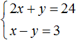
Add the left side of the first equation to the left side of the second equation. And the right side of the first equation with the right side of the second equation. We get the following equality:

Here are similar terms:

As a result, we obtained the simplest equation 3 x= 27 whose root is 9. Knowing the value x you can find the value y. Substitute the value x into the second equation x − y= 3 . We get 9 − y= 3 . From here y= 6 .

So the solution of the system is a pair of values ​​(9; 6)

Example 2

Add the left side of the first equation to the left side of the second equation. And the right side of the first equation with the right side of the second equation. In the resulting equality, we present like terms:

As a result, we got the simplest equation 5 x= 20, the root of which is 4. Knowing the value x you can find the value y. Substitute the value x into the first equation 2 x+y= 11 . Let's get 8 + y= 11 . From here y= 3 .

So the solution of the system is the pair of values ​​(4;3)

The addition process is not described in detail. It has to be done in the mind. When adding, both equations must be reduced to canonical form. That is, to the mind ac+by=c .

From the considered examples, it can be seen that the main goal of adding equations is to get rid of one of the variables. But it is not always possible to immediately solve the system of equations by the addition method. Most often, the system is preliminarily brought to a form in which it is possible to add the equations included in this system.

For example, the system can be solved directly by the addition method. When adding both equations, the terms y and −y vanish because their sum is zero. As a result, the simplest equation is formed 11 x= 22 , whose root is 2. Then it will be possible to determine y equal to 5.

And the system of equations the addition method cannot be solved immediately, since this will not lead to the disappearance of one of the variables. Addition will result in Equation 8 x+ y= 28 , which has an infinite number of solutions.

If both parts of the equation are multiplied or divided by the same number that is not equal to zero, then an equation equivalent to the given one will be obtained. This rule is also valid for a system of linear equations with two variables. One of the equations (or both equations) can be multiplied by some number. The result is an equivalent system, the roots of which will coincide with the previous one.

Let's return to the very first system, which described how many cakes and cups of coffee the student bought. The solution of this system was a pair of values ​​(6; 5) .

We multiply both equations included in this system by some numbers. Let's say we multiply the first equation by 2 and the second by 3

The result is a system
The solution to this system is still the pair of values ​​(6; 5)

This means that the equations included in the system can be reduced to a form suitable for applying the addition method.

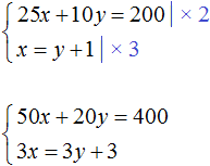
Back to the system , which we could not solve by the addition method.

Multiply the first equation by 6 and the second by −2

Then we get the following system:

We add the equations included in this system. Addition of components 12 x and -12 x will result in 0, addition 18 y and 4 y will give 22 y, and adding 108 and −20 gives 88. Then you get the equation 22 y= 88 , hence y = 4 .

If at first it is difficult to add equations in your mind, then you can write down how the left side of the first equation is added to the left side of the second equation, and the right side of the first equation to the right side of the second equation:

Knowing that the value of the variable y is 4, you can find the value x. Substitute y into one of the equations, for example into the first equation 2 x+ 3y= 18 . Then we get an equation with one variable 2 x+ 12 = 18 . We transfer 12 to the right side, changing the sign, we get 2 x= 6 , hence x = 3 .

Example 4. Solve the following system of equations using the addition method:

Multiply the second equation by −1. Then the system will take the following form:

Let's add both equations. Addition of components x and −x will result in 0, addition 5 y and 3 y will give 8 y, and adding 7 and 1 gives 8. The result is equation 8 y= 8 , whose root is 1. Knowing that the value y is 1, you can find the value x .

Substitute y into the first equation, we get x+ 5 = 7 , hence x= 2

Example 5. Solve the following system of equations using the addition method:

It is desirable that the terms containing the same variables are located one under the other. Therefore, in the second equation, the terms 5 y and −2 x change places. As a result, the system will take the form:

Multiply the second equation by 3. Then the system will take the form:

Now let's add both equations. As a result of addition, we get equation 8 y= 16 , whose root is 2.

Substitute y into the first equation, we get 6 x− 14 = 40 . We transfer the term −14 to the right side, changing the sign, we get 6 x= 54 . From here x= 9.

Example 6. Solve the following system of equations using the addition method:

Let's get rid of fractions. Multiply the first equation by 36 and the second by 12

In the resulting system the first equation can be multiplied by −5 and the second by 8

Let's add the equations in the resulting system. Then we get the simplest equation −13 y= −156 . From here y= 12 . Substitute y into the first equation and find x

Example 7. Solve the following system of equations using the addition method:

We bring both equations to normal form. Here it is convenient to apply the rule of proportion in both equations. If in the first equation the right side is represented as , and the right side of the second equation as , then the system will take the form:

We have a proportion. We multiply its extreme and middle terms. Then the system will take the form:

We multiply the first equation by −3, and open the brackets in the second:

Now let's add both equations. As a result of adding these equations, we get an equality, in both parts of which there will be zero:

It turns out that the system has an infinite number of solutions.

But we cannot simply take arbitrary values ​​from the sky for x and y. We can specify one of the values, and the other will be determined depending on the value we specify. For example, let x= 2 . Substitute this value into the system:

As a result of solving one of the equations, the value for y, which will satisfy both equations:

The resulting pair of values ​​(2; −2) will satisfy the system:

Let's find another pair of values. Let x= 4. Substitute this value into the system:

It can be determined by eye that y equals zero. Then we get a pair of values ​​(4; 0), which satisfies our system:

Example 8. Solve the following system of equations using the addition method:

Multiply the first equation by 6 and the second by 12

Let's rewrite what's left:

Multiply the first equation by −1. Then the system will take the form:

Now let's add both equations. As a result of addition, equation 6 is formed b= 48 , whose root is 8. Substitute b into the first equation and find a

System of linear equations with three variables

A linear equation with three variables includes three variables with coefficients, as well as an intercept. In canonical form, it can be written as follows:

ax + by + cz = d

This equation has an infinite number of solutions. By giving two variables different values, a third value can be found. The solution in this case is the triple of values ​​( x; y; z) which turns the equation into an identity.

If variables x, y, z are interconnected by three equations, then a system of three linear equations with three variables is formed. To solve such a system, you can apply the same methods that apply to linear equations with two variables: the substitution method and the addition method.

Example 1. Solve the following system of equations using the substitution method:

We express in the third equation x. Then the system will take the form:

Now let's do the substitution. Variable x is equal to the expression 3 − 2y − 2z . Substitute this expression into the first and second equations:

Let's open the brackets in both equations and give like terms:

We have arrived at a system of linear equations with two variables. In this case, it is convenient to apply the addition method. As a result, the variable y will disappear and we can find the value of the variable z

Now let's find the value y. For this, it is convenient to use the equation − y+ z= 4. Substitute the value z

Now let's find the value x. For this, it is convenient to use the equation x= 3 − 2y − 2z . Substitute the values ​​into it y and z

Thus, the triple of values ​​(3; −2; 2) is the solution to our system. By checking, we make sure that these values ​​​​satisfy the system:

Example 2. Solve the system by addition method

Let's add the first equation with the second multiplied by −2.

If the second equation is multiplied by −2, then it will take the form −6x+ 6y- 4z = −4 . Now add it to the first equation:

We see that as a result of elementary transformations, the value of the variable was determined x. It is equal to one.

Let's go back to the main system. Let's add the second equation with the third multiplied by −1. If the third equation is multiplied by −1, then it will take the form −4x + 5y − 2z = −1 . Now add it to the second equation:

Got the equation x - 2y= −1 . Substitute the value into it x which we found earlier. Then we can determine the value y

We now know the values x and y. This allows you to determine the value z. We use one of the equations included in the system:

Thus, the triple of values ​​(1; 1; 1) is the solution to our system. By checking, we make sure that these values ​​​​satisfy the system:

Tasks for compiling systems of linear equations

The task of compiling systems of equations is solved by introducing several variables. Next, equations are compiled based on the conditions of the problem. From the compiled equations, they form a system and solve it. Having solved the system, it is necessary to check whether its solution satisfies the conditions of the problem.

Task 1. A Volga car left the city for the collective farm. She returned back along another road, which was 5 km shorter than the first. In total, the car drove 35 km both ways. How many kilometers is each road long?

Solution

Let x- length of the first road, y- the length of the second. If the car drove 35 km both ways, then the first equation can be written as x+ y= 35. This equation describes the sum of the lengths of both roads.

It is said that the car was returning back along the road, which was shorter than the first one by 5 km. Then the second equation can be written as x− y= 5. This equation shows that the difference between the lengths of the roads is 5 km.

Or the second equation can be written as x= y+ 5 . We will use this equation.

Since the variables x and y in both equations denote the same number, then we can form a system from them:

Let's solve this system using one of the previously studied methods. In this case, it is convenient to use the substitution method, since in the second equation the variable x already expressed.

Substitute the second equation into the first and find y

Substitute the found value y into the second equation x= y+ 5 and find x

The length of the first road was denoted by the variable x. Now we have found its meaning. Variable x is 20. So the length of the first road is 20 km.

And the length of the second road was indicated by y. The value of this variable is 15. So the length of the second road is 15 km.

Let's do a check. First, let's make sure that the system is solved correctly:

Now let's check whether the solution (20; 15) satisfies the conditions of the problem.

It was said that in total the car drove 35 km both ways. We add up the lengths of both roads and make sure that the solution (20; 15) satisfies this condition: 20 km + 15 km = 35 km

Next condition: the car returned back along another road, which was 5 km shorter than the first . We see that the solution (20; 15) also satisfies this condition, since 15 km is shorter than 20 km by 5 km: 20 km − 15 km = 5 km

When compiling a system, it is important that the variables denote the same numbers in all equations included in this system.

So our system contains two equations. These equations in turn contain the variables x and y, which denote the same numbers in both equations, namely the lengths of roads equal to 20 km and 15 km.

Task 2. Oak and pine sleepers were loaded onto the platform, a total of 300 sleepers. It is known that all oak sleepers weighed 1 ton less than all pine sleepers. Determine how many oak and pine sleepers there were separately, if each oak sleeper weighed 46 kg, and each pine sleeper 28 kg.

Solution

Let x oak and y pine sleepers were loaded onto the platform. If there were 300 sleepers in total, then the first equation can be written as x+y = 300 .

All oak sleepers weighed 46 x kg, and pine weighed 28 y kg. Since oak sleepers weighed 1 ton less than pine sleepers, the second equation can be written as 28y- 46x= 1000 . This equation shows that the mass difference between oak and pine sleepers is 1000 kg.

Tons have been converted to kilograms because the mass of oak and pine sleepers is measured in kilograms.

As a result, we obtain two equations that form the system

Let's solve this system. Express in the first equation x. Then the system will take the form:

Substitute the first equation into the second and find y

Substitute y into the equation x= 300 − y and find out what x

This means that 100 oak and 200 pine sleepers were loaded onto the platform.

Let's check whether the solution (100; 200) satisfies the conditions of the problem. First, let's make sure that the system is solved correctly:

It was said that there were 300 sleepers in total. We add up the number of oak and pine sleepers and make sure that the solution (100; 200) satisfies this condition: 100 + 200 = 300.

Next condition: all oak sleepers weighed 1 ton less than all pine . We see that the solution (100; 200) also satisfies this condition, since 46 × 100 kg of oak sleepers are lighter than 28 × 200 kg of pine sleepers: 5600 kg − 4600 kg = 1000 kg.

Task 3. We took three pieces of an alloy of copper and nickel in ratios of 2: 1, 3: 1 and 5: 1 by weight. Of these, a piece weighing 12 kg was fused with a ratio of copper and nickel content of 4: 1. Find the mass of each original piece if the mass of the first of them is twice the mass of the second.

The material of this article is intended for the first acquaintance with systems of equations. Here we introduce the definition of a system of equations and its solutions, and also consider the most common types of systems of equations. As usual, we will give explanatory examples.

Page navigation.

What is a system of equations?

We will gradually approach the definition of the system of equations. At first, we will only say that it is convenient to give it, pointing out two points: firstly, the type of record, and, secondly, the meaning embedded in this record. Let us dwell on them in turn, and then generalize the reasoning into the definition of systems of equations.

Let us have some of them in front of us. For example, let's take two equations 2 x+y=−3 and x=5 . We write them one under the other and unite them with a curly bracket on the left:

Records of this kind, which are several equations arranged in a column and united on the left with a curly bracket, are records of systems of equations.

What do such records mean? They define the set of all such solutions of the equations of the system, which are the solution of each equation.

It does not hurt to describe it in other words. Suppose some solutions of the first equation are solutions of all other equations of the system. And so record of system just also designates them.

Now we are ready to adequately accept the definition of a system of equations.

Definition.

Systems of equations are called records, which are equations located one below the other, united on the left by a curly bracket, which denote the set of all solutions of equations that are simultaneously solutions to each equation of the system.

A similar definition is given in the textbook, but there it is given not for the general case, but for two rational equations with two variables.

Main types

It is clear that there are infinitely many different equations. Naturally, there are also infinitely many systems of equations compiled using them. Therefore, for the convenience of studying and working with systems of equations, it makes sense to divide them into groups according to similar characteristics, and then proceed to consider systems of equations of individual types.

The first subdivision suggests itself by the number of equations included in the system. If there are two equations, then we can say that we have a system of two equations, if there are three, then a system of three equations, etc. It is clear that it makes no sense to talk about a system of one equation, since in this case, in fact, we are dealing with the equation itself, and not with the system.

The next division is based on the number of variables involved in writing the equations of the system. If there is one variable, then we are dealing with a system of equations with one variable (they also say with one unknown), if there are two, then with a system of equations with two variables (with two unknowns), etc. For example, is a system of equations with two variables x and y .

This refers to the number of all different variables involved in the record. They do not have to be all at once included in the record of each equation, it is enough to have them in at least one equation. For example, is a system of equations with three variables x, y, and z. In the first equation, the variable x is present explicitly, while y and z are implicit (we can assume that these variables have zero), and in the second equation, x and z are present, and the variable y is not explicitly represented. In other words, the first equation can be viewed as , and the second as x+0 y−3 z=0 .

The third point in which systems of equations differ is the form of the equations themselves.

At school, the study of systems of equations begins with systems of two linear equations in two variables. That is, such systems constitute two linear equations. Here are a couple of examples: and . On them, the basics of working with systems of equations are learned.

When solving more complex problems, one can also encounter systems of three linear equations with three unknowns.

Further in the 9th grade, non-linear equations are added to the systems of two equations with two variables, for the most part entire equations of the second degree, less often - of higher degrees. These systems are called systems of nonlinear equations; if necessary, the number of equations and unknowns is specified. Let us show examples of such systems of nonlinear equations: and .

And then in the systems there are also, for example,. They are usually called simply systems of equations, without specifying which equations. Here it is worth noting that most often they simply say “system of equations” about a system of equations, and refinements are added only if necessary.

In high school, as the material is studied, irrational, trigonometric, logarithmic and exponential equations penetrate into the systems: , , .

If you look even further into the program of the first courses of universities, then the main emphasis is on the study and solution of systems of linear algebraic equations (SLAE), that is, equations, in the left parts of which are polynomials of the first degree, and in the right - some numbers. But there, unlike the school, not two linear equations with two variables are already taken, but an arbitrary number of equations with an arbitrary number of variables, often not coinciding with the number of equations.

What is the solution of a system of equations?

The term “solution of a system of equations” directly refers to systems of equations. The school gives a definition of solving a system of equations with two variables :

Definition.

Solving a system of equations with two variables a pair of values ​​of these variables is called, which turns each equation of the system into the correct one, in other words, which is the solution to each equation of the system.

For example, a pair of variable values ​​x=5 , y=2 (it can be written as (5, 2) ) is a solution to a system of equations by definition, since the equations of the system, when x=5 , y=2 are substituted into them, turn into true numerical equalities 5+2=7 and 5−2=3 respectively. But the pair of values ​​x=3 , y=0 is not a solution to this system, since when these values ​​are substituted into the equations, the first of them will turn into an incorrect equality 3+0=7 .

Similar definitions can be formulated for systems with one variable, as well as for systems with three, four, etc. variables.

Definition.

Solving a system of equations with one variable there will be a variable value that is the root of all the equations of the system, that is, that turns all equations into true numerical equalities.

Let's take an example. Consider a system of equations with one variable t of the form . The number −2 is its solution, since both (−2) 2 =4 and 5·(−2+2)=0 are true numerical equalities. And t=1 is not a solution to the system, since substitution of this value will give two incorrect equalities 1 2 =4 and 5·(1+2)=0 .

Definition.

The solution of a system with three, four, etc. variables called a triple, a quadruple, etc. values ​​of the variables, respectively, which converts all equations of the system into true equalities.

So, by definition, the triple of values ​​of the variables x=1 , y=2 , z=0 is the solution to the system , since 2 1=2 , 5 2=10 and 1+2+0=3 are correct numerical equalities. And (1, 0, 5) is not a solution to this system, since when these values ​​of variables are substituted into the equations of the system, the second of them turns into an incorrect equality 5 0=10 , and the third one is also 1+0+5=3 .

Note that systems of equations may not have solutions, may have a finite number of solutions, for example, one, two, ..., or may have infinitely many solutions. You will see this as you delve deeper into the topic.

Taking into account the definitions of a system of equations and their solutions, we can conclude that the solution of a system of equations is the intersection of the sets of solutions of all its equations.

To conclude, here are a few related definitions:

Definition.

incompatible if it has no solutions, otherwise the system is called joint.

Definition.

The system of equations is called uncertain if it has infinitely many solutions, and certain, if it has a finite number of solutions, or has none at all.

These terms are introduced, for example, in a textbook, but they are rarely used at school, more often they can be heard in higher educational institutions.

Bibliography.

1. Algebra: textbook for 7 cells. general education institutions / [Yu. N. Makarychev, N. G. Mindyuk, K. I. Neshkov, S. B. Suvorova]; ed. S. A. Telyakovsky. - 17th ed. - M. : Education, 2008. - 240 p. : ill. - ISBN 978-5-09-019315-3.
2. Algebra: Grade 9: textbook. for general education institutions / [Yu. N. Makarychev, N. G. Mindyuk, K. I. Neshkov, S. B. Suvorova]; ed. S. A. Telyakovsky. - 16th ed. - M. : Education, 2009. - 271 p. : ill. - ISBN 978-5-09-021134-5.
3. Mordkovich A. G. Algebra. 7th grade. At 2 pm Part 1. A textbook for students of educational institutions / A. G. Mordkovich. - 17th ed., add. - M.: Mnemozina, 2013. - 175 p.: ill. ISBN 978-5-346-02432-3.
4. Mordkovich A. G. Algebra. Grade 9 At 2 pm Part 1. Textbook for students of educational institutions / A. G. Mordkovich, P. V. Semenov. - 13th ed., Sr. - M.: Mnemosyne, 2011. - 222 p.: ill. ISBN 978-5-346-01752-3.
5. Mordkovich A. G. Algebra and beginning of mathematical analysis. Grade 11. At 2 pm Part 1. Textbook for students of educational institutions (profile level) / A. G. Mordkovich, P. V. Semenov. - 2nd ed., erased. - M.: Mnemosyne, 2008. - 287 p.: ill. ISBN 978-5-346-01027-2.
6. Algebra and the beginning of the analysis: Proc. for 10-11 cells. general education institutions / A. N. Kolmogorov, A. M. Abramov, Yu. P. Dudnitsyn and others; Ed. A. N. Kolmogorova.- 14th ed.- M.: Enlightenment, 2004.- 384 p.: ill.- ISBN 5-09-013651-3.
7. A. G. Kurosh. Course of higher algebra.
8. Ilyin V. A., Poznyak E. G. Analytic geometry: Textbook: For universities. – 5th ed. – M.: Science. Fizmatlit, 1999. - 224 p. – (Course of higher mathematics and mathematical physics). – ISBN 5-02-015234 – X (Issue 3)